

I use Excel… a LOT, and for a very long time! With that comes the inevitable… my eyes aren’t as young as they used to be… plus, we tend to have a TON of data in our Excel file, sometimes making it harder to know which data is on the row that I am looking at.
I know, you can use themes, or highlight the row manually, but I want something dynamic. I want to highlight the active row (the row where my cursor is)… and I am greedy, I want it to change every time I change rows.
I personally think this should be a feature built into Excel, but I cannot find it anywhere – if you know of a different way, please post a comment below.
I’ve put together a few steps to automatically highlight my active row. Read on to see these steps and maybe put it to use for you!
The video below may take a moment to load – give it just a minute please – for some reason, wordpress doesn’t play well with ‘Gifs’. Comment below and let me know if you like this tip!

To highlight the row you are working on, there are a few steps you need to go through for the file. In addition, you should know in advance, the file will need to become a macro file (xlsm) because we will be adding a tiny bit of VBA – DON’T WORRY!! This is easy, so keep reading!
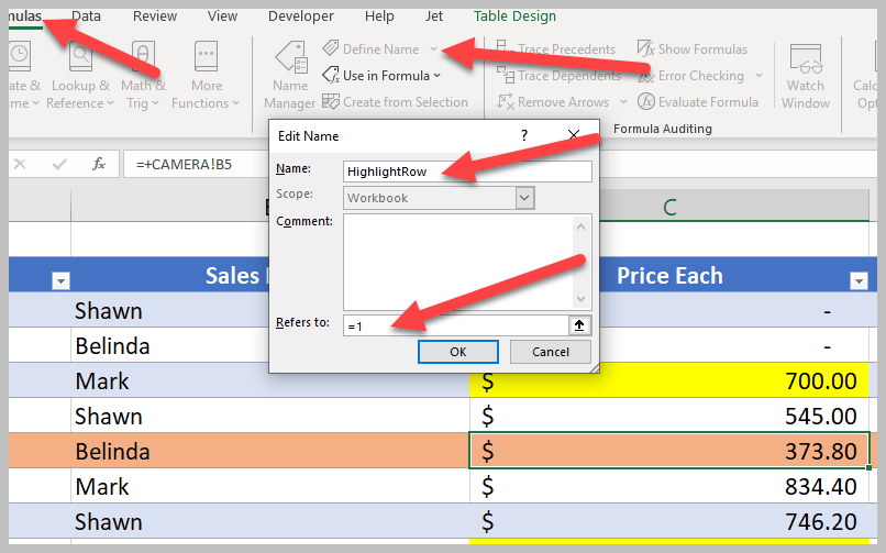
Step 1: Define a Name Range to use in VBA
A named range is needed – to do this, just go to Formulas/Define Name. I used ‘HighlightRow’ as my name. You can use whatever you would like, but it must be used later, so be sure to be consistent.
Also, the ‘REFERS TO’ box must be changed to ‘=1’.
Step 2: Add Conditional Formatting
In this step, we will need to add the conditional formatting that will be used in our VBA.
Click the ‘select all cells’ button in the top left of your spreadsheet.

Next, go to the Home Tab, then go to conditional formatting, and add a new rule.

When the new Formatting Rule window opens, choose ‘Use a Formula’ and then define the formula. The formula will be ‘=Row(a1)=HighlightRow’ – where “HighlightRow” is the name of the defined range in Step 1. Then click the format button.

In the format cells window, switch to the fill tab, and choose the color you want to use as the color to highlight the active row.

Then click OK on the Format Cells window, and OK on the New Formatting Rule window. At this point, Row 1 should be highlighted with the color you selected. But that’s not the complete end result that we want… we want the row to change when our active row changes. This is where we bring in a little VBA.
Step 3: Add VBA
For this step, you will need the Developer tab available in your ribbon. If it is not available, you can add it by going to File/Options/Customize Ribbon and turn on the developers tab.

In the developer tab, click Visual Basic. This will open the Visual Basic Editor. Select the workbook you are working on, and double click the sheet you want this code to work with… When you double click, the code window will open, change the drop down from General to Worksheet.

Once you select worksheet from the drop down, be sure that the second drop down shows ‘SelectionChange’ is selected, if not, use the drop down and select it.
The default code will look like this:
Private Sub Worksheet_SelectionChange(ByVal Target As Range)
End Sub
Highlight the default code and replace it with this:
Private Sub Worksheet_SelectionChange(ByVal Target As Range)
With ThisWorkbook.Names("HighlightRow")
.Name = "HighlightRow"
.RefersToR1C1 = "=" & ActiveCell.Row
End With
End Sub
In the code above, be sure that the value in quotes (“HighlightRow”) matches your named range that you defined in step 1.

Close the VBA window and go back to excel. If you followed the steps closely, you should be able to change active cells and have them automatically highlight! VERY VERY COOL!!
Step 4: Save as xlsm file
If you do not save this Excel file as an xlsm file, the code will only work this one time. In order to keep the VBA, save it as an XLSM file (Macro) and it will work every time you open the file up! Simply go to File, Save as, and choose the drop down for macro files.

That’s it! You are all set! YOU DID IT!!! Now, go impress your friend!!! 🙂
The image right above this line is a GIF file of this change in action (if you do not see it, try opening this page up on a desktop) – I want to make sure to thank my friend, and fellow MVP, Jen Kuntz for motivating me to use a GIF – it’s my first time, thanks Jen!! Jen adds to her own blog EVERY TUESDAY – be sure to check it out here.
Pretty Cool huh? I use this a lot and I hope you enjoy it!
I learned how to do this by combining a few things I found across the web… I do not write VBA – I did it, so you can too!!
Thanks for reading!
Shawn Dorward
Microsoft MVP, Business Applications
LifeHacks365.com | LinkedIn | Twitter
Is there a way to make this work across two worksheets within the same workbook? I’ve been using this tip every single day for many months now and it has greatly improved my life. I would love to be able to highlight the active row on additional sheets though. Thank you!
This worked great but I realized that now I can’t use the undo anymore. After some googling apparently once you run a VBA you can no longer use Undo. I need undo more than this feature so now I have to figure out how to remove it.
Hi thanks a lot! it is amazing!
However, could the code be altered so all rows that contains duplicated values (in column C for example) could be highlighted as well?
OMG!! Happiness is when I find a “fix” and it ACTUALLY WORKS!!!!!
Just stumbled upon this now and definitely helpful. Thank you good sir!
Very cool. Thanks for posting these great instructions. Worked the first time.
Hello! I would also like to know how to duplicate this across all sheets in a workbook! Thanks
I want to know the same!
Really appreciate this! I have a table of data that will grow by about 100 rows per day. My boss wanted every other row to highlight, to make data entry easier. But having the table grow meant it would be cumbersome to pre-color those rows. And the table is heavily macro driven, and sometimes Excel Tables do not play well with macros. This solved my problem. Many thanks!
Thank you very much! This is such a great help!
This helped so much. Thanks
Awesome, super useful hack! The instructions are very clear and easy to follow, even for an excel novice such as myself. Thank you!!!
(I have been copying lots of data from one excel to another, using two screens and with plenty of edits and data double checking. This was exactly what I needed to help my poor eyeballs and avoid silly mistakes)
Thanks for this hack. I got it to work on my Excel 2016. I just had to adjust the VBA code part.
Private Sub Worksheet_SelectionChange(ByVal Target As Range)
Dim ws As Worksheet
Set ws = Sheets(“HighlightRow”)
ws.Names.Item(“HighlightRow”).RefersToR1C1 = “=” & ActiveCell.row
End Sub
Doesnt seem to work for me and only highlights Row A1. Does anyone know why??
Thank you! Step by step directions were simple to follow and IT WORKED!
Wow!
I feel like an expert now.
This will be a great tool when I’m looking at a file with large data.
TYSM
I’m a little late to the game, but this is pretty awesome. I did have one issue I’m trying to figure out, wondering if anybody has come across this. When I have a table filtered it seems to break this functionality. It will actually still highlight a row, but it will not be the row that I’ve selected. Anyone have any ideas?
Thank you thank you thank you!!!!!!
It worked! Hell yeah! Thanks, man!
Hi,
Thanks so much for this tips. It’s made my life so much easier
Hi ! I know very little about VBA.
I have a workbook with about 10 worksheets
I am attempting to use your highlight row code for the worksheet named INS
I am getting an error for this line, hoping you can assist 🙂
With ThisWorkbook.Names(“HighlightRow”)
Private Sub Worksheet_SelectionChange(ByVal Target As Range)
With ThisWorkbook.Names(“HighlightRow”)
.Name = “HighlightRow”
.RefersToR1C1 = “=” & ActiveCell.Row
End With
End Sub
I am also using another code that i found on the web to active cell A1 on open:
Private Sub Workbook_Open()
Dim WSheet As Worksheet
For Each WSheet In Worksheets
WSheet(“INS”).Activate
WSheet.Activate
Range(“A1”).Select
Next
End Sub
Tmirelle,
What is the error that you see? The code looks identical to the code in Shawn’s article.
Did you define the Named Range (HighlightRow) in Formulas >> Name Manager?
Steve Erbach
I was getting an error too, with the following line:
> With ThisWorkbook.Names(“HighlightRow”)
The error message was:
> Run-time error ‘1004’:
> Method ‘_Default’ of object ‘Names’ failed
I realised when I created the name “HighlightRow” in the Names manager, I chose to make the name on the current worksheet instead of the entire workbook. This was intentional, but I didn’t anticipate it would cause a problem. It was an easy fix, I just specified which worksheet the “HighlightRow” name was part of:
> With ThisWorkbook.ActiveSheet.Names(“HighlightRow”)
If you wanted to be more specific (rather than using .ActiveSheet) you can use the following instead:
> With ThisWorkbook.Sheets(“NAME-OF-WORKSHEET”).Names(“HighlightRow”)
Also, since I was using Excel for Mac, I was initially getting a separate error whenever I tried to change the VBA drop-down from “(General)” to “Worksheet”:
> Variable uses an Automation type not supported in Visual Basic
This was easily remedied by ignoring that step (leaving the drop-down on “(General)”, unchanged) and simply pasting in the entire code on this blog post. Basically, typing the following automatically changes the VBA drop-down to “Worksheet” regardless:
> Private Sub Worksheet_SelectionChange(ByVal Target As Range)
>
> End Sub
I had the same issue because I was using the code for a specific sheet not the workbook. Change
With ThisWorkbook.Names(“HighlightRow”)
With Worksheets(“INS”).Names(“HighlightRow”)
Perfect.
Brilliant. Worked perfectly. Thank you!
This looks great, however it seems to disable the Undo function. I’ll check some more into this and hopefully have a comment later,
What a legend. Kudos on also the proper screenshots so we could skim quickly. Wish every hack was like this.
Hi, this worked like magic! Thank you SO MUCH!
Is there a way to modify this to highlight several selected rows?
Worked like a dream!
Thank you so very much for this! As others have stated too, it really is life-changing for people who work in spreadsheets a lot. It is really generous and wonderful of you to share this – thank you!
What I noticed is that if you move the “highlighted bar” after entering something, there is no undo possible anymore.
Can I apply this to more than a single worksheet within a workbook? I have a spreadsheet with three tabs (worksheets) and I’d like this to work on all three worksheets.
Did you got your answer for three work sheets ?
Thank you! Worked perfectly. Is it possible to have my pre-exisitng cell colours show through at all?
Hello. This works perfectly to highlight the active row. I often have 2 very large spreadsheets open at the same time and have to compare data. The highlights help me to easily find my place. The only problem I am having is when I copy data from one spreadsheet to another. I get this warning: “The name ‘HighlightRow’ already exists. Click Yes to use that version of the name, or click No to rename the version of ‘HighlightRow’ you’re moving or copying.” If I click Yes, the data pastes in but I get that warning every single time I copy and paste into a different spreadsheet. If I click No and rename ‘HighlightRow’, the data pastes in but the next time I copy and paste I get the same warning. Is there a solution? Thank you.
Hi Shawn,
Great code and article. Very easy to follow.
Wondering if it’s possible that the conditional formatting can be excluded from the active cell but the active row remains highlighted?
Worked perfectly. Thanks!
This has got to be the easiest step by step (with examples) that I have every run into. Even this ancient of days got it done in very little time. Now looking forward to see how it can be modified/adjusted to apply to a work-book, not just the sheet. Anyway, thanks so much for the help. have signed up for the new posts. JFS.
HighlighCell? Is there a way to modify this so that it highlights the active cell instead of the entire row?
Thank you for the code. How do I activate this for the entire workbook? I have 15 worksheets.
I agree with most of the comments. It was easy to follow. Can you apply this same rule for a column? Having a row and column highlighted with the cursor in the cross cell would be great!
Hi – just want to say thank you!!!! This should be a standard ON/OFF feature in Excel. Thank you
I followed everything but its not working for me. There’s no error but the highlight doesnt work.
I have never written any code in Excel before – I just followed all the instructions given on this page and it worked!
It is working fantastically, in fact!! This comes in handy so much when you are working on two workbooks where you need to transfer date from one to the other, helps so much to keep track of your position and contents.
Thank you for sharing this amazing trick @Shawn Dorward !
I’m in the same boat as Stefan. I con no longer use the undo function in excel. This work around will not be worth it if something as simple as clicking undo can no longer be used.
For me, it seems to highlight the row 12 under my selection and I can’t figure out why.
How can I make the code work for different worksheet within the same file so it differs and doesn’t highlight the same row for all the worksheets?
This is Great, however my excel is highlighting the row 24 rows under my selected cell. Could anyone help me with some trouble shooting?
undo doesn’t work because it is a macro see https://www.quora.com/Has-the-Undo-button-in-Microsoft-Excel-stopped-working