

I use Excel… a LOT, and for a very long time! With that comes the inevitable… my eyes aren’t as young as they used to be… plus, we tend to have a TON of data in our Excel file, sometimes making it harder to know which data is on the row that I am looking at.
I know, you can use themes, or highlight the row manually, but I want something dynamic. I want to highlight the active row (the row where my cursor is)… and I am greedy, I want it to change every time I change rows.
I personally think this should be a feature built into Excel, but I cannot find it anywhere – if you know of a different way, please post a comment below.
I’ve put together a few steps to automatically highlight my active row. Read on to see these steps and maybe put it to use for you!
The video below may take a moment to load – give it just a minute please – for some reason, wordpress doesn’t play well with ‘Gifs’. Comment below and let me know if you like this tip!

To highlight the row you are working on, there are a few steps you need to go through for the file. In addition, you should know in advance, the file will need to become a macro file (xlsm) because we will be adding a tiny bit of VBA – DON’T WORRY!! This is easy, so keep reading!
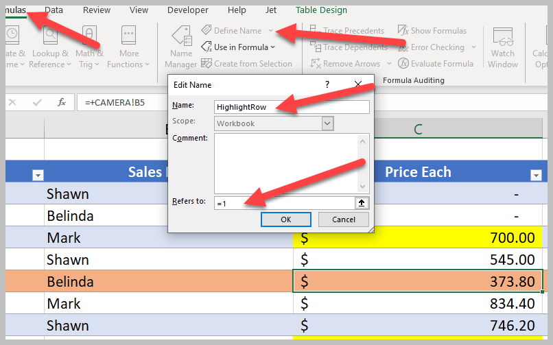
Step 1: Define a Name Range to use in VBA
A named range is needed – to do this, just go to Formulas/Define Name. I used ‘HighlightRow’ as my name. You can use whatever you would like, but it must be used later, so be sure to be consistent.
Also, the ‘REFERS TO’ box must be changed to ‘=1’.
Step 2: Add Conditional Formatting
In this step, we will need to add the conditional formatting that will be used in our VBA.
Click the ‘select all cells’ button in the top left of your spreadsheet.

Next, go to the Home Tab, then go to conditional formatting, and add a new rule.

When the new Formatting Rule window opens, choose ‘Use a Formula’ and then define the formula. The formula will be ‘=Row(a1)=HighlightRow’ – where “HighlightRow” is the name of the defined range in Step 1. Then click the format button.

In the format cells window, switch to the fill tab, and choose the color you want to use as the color to highlight the active row.

Then click OK on the Format Cells window, and OK on the New Formatting Rule window. At this point, Row 1 should be highlighted with the color you selected. But that’s not the complete end result that we want… we want the row to change when our active row changes. This is where we bring in a little VBA.
Step 3: Add VBA
For this step, you will need the Developer tab available in your ribbon. If it is not available, you can add it by going to File/Options/Customize Ribbon and turn on the developers tab.

In the developer tab, click Visual Basic. This will open the Visual Basic Editor. Select the workbook you are working on, and double click the sheet you want this code to work with… When you double click, the code window will open, change the drop down from General to Worksheet.

Once you select worksheet from the drop down, be sure that the second drop down shows ‘SelectionChange’ is selected, if not, use the drop down and select it.
The default code will look like this:
Private Sub Worksheet_SelectionChange(ByVal Target As Range)
End Sub
Highlight the default code and replace it with this:
Private Sub Worksheet_SelectionChange(ByVal Target As Range)
With ThisWorkbook.Names("HighlightRow")
.Name = "HighlightRow"
.RefersToR1C1 = "=" & ActiveCell.Row
End With
End Sub
In the code above, be sure that the value in quotes (“HighlightRow”) matches your named range that you defined in step 1.

Close the VBA window and go back to excel. If you followed the steps closely, you should be able to change active cells and have them automatically highlight! VERY VERY COOL!!
Step 4: Save as xlsm file
If you do not save this Excel file as an xlsm file, the code will only work this one time. In order to keep the VBA, save it as an XLSM file (Macro) and it will work every time you open the file up! Simply go to File, Save as, and choose the drop down for macro files.

That’s it! You are all set! YOU DID IT!!! Now, go impress your friend!!! 🙂
The image right above this line is a GIF file of this change in action (if you do not see it, try opening this page up on a desktop) – I want to make sure to thank my friend, and fellow MVP, Jen Kuntz for motivating me to use a GIF – it’s my first time, thanks Jen!! Jen adds to her own blog EVERY TUESDAY – be sure to check it out here.
Pretty Cool huh? I use this a lot and I hope you enjoy it!
I learned how to do this by combining a few things I found across the web… I do not write VBA – I did it, so you can too!!
Thanks for reading!
Shawn Dorward
Microsoft MVP, Business Applications
LifeHacks365.com | LinkedIn | Twitter
Shawn, your steps are very easy to follow. I do believe that I was able to follow them to the letter, however I keep getting a VBA erro message saying that the subscript is out of range even though the HighlightRow is what I named the defined range in step 1. What am I doing wrong?
Lori – if you see Steve’s comment below, he is pointing out EXACTLY what is causing your error – I reposted the code in my blog so trying to copy and paste it should work now. Otherwise, replace the quotes per Steve’s note and remove the spaces around the = sign 🙂 Please post back and let us know if this works!
Hi, Shawn! I am shamelessly using this method to show to our GPUG Chapter. There are a couple things to watch out for with the Sub Worksheet_SelectionChange() code above.
1. If you copy and paste the code directly from the web page into your VBA editor, the quotation marks surrounding the “HighlightRow” and the “=” sign are ACTUAL open and close quotation marks, which VBA doesn’t recognize. You have to replace them all with the plain-jane ” mark.
2. In the pasted code in the VBA editor, the “=” winds up actually being ” = “. There’s a space before and after the = sign. VBA doesn’t like that either.
Once those two things are taken care of in the code, the highlight works!
Thanks Steve!! Glad it was helpful! I noted your changes into my blog post so they should work as copied now – give it a shot and let me know 🙂 Thanks so much!
That’s just the ticket, Shawn!
By the way, during my presentation of this method at our GPUG Green Bay Chapter meeting yesterday, one of our members pointed out that one can always click on the row number to highlight the whole row. While that’s true, I replied, as soon as you click on any cell in that row, the highlight goes away. Your method leaves the highlight intact so that you don’t lose your place! And it works from anywhere in the sheet, mouse or keyboard.
The only shortcoming is that, apparently, one must activate this code for each sheet in a workbook. Is this the case?
Thanks for making the correction… and thanks even more for this cool tip!
This hack is life! I can’t express how greatful I am to have found this and how easy it was to complete. You ROCK!
Thanks Cindy!! SO GLAD IT HELPED!!
I love it! I added this in to one of my most used workbooks. Is there a way to save this as a macro that works on all spreadsheets, or does this have to be done one spreadsheet at a time?
Thanks Stefanie! I’m glad you enjoy this lifehack! I am not aware of a way to have it work on more than one spreadsheet at a time but it is on my list to investigate 🙂
Hello Stefanie & Shawn,
You just need to apply this hack on a new empty excel file and save it as a default template. The next time you create a new workbook, you’ll get what you want.
Just google “How to set a default template in Excel” and you’ll find detailed steps 😉
Or you just hit Shift + Space
Shift+Space highlights the row but it doesn’t keep it highlighted if you move your cursor. The method above keeps it highlighted, which for me, helps a lot! 🙂 Thank you for visiting!
And, most importantly, when you are using Find & Replace, Row can be easily noticed with this vba formula. Thanks!
Thank you for this, after a small modifications (language french, replace Row–>Ligne) it worked perfectly
So very helpful. Many thanks!
Hi Shawn! I’d like to be able to highlight multiple rows having the same value of the selected cell. Do you know of a way to do that?
Thank you in advance
Although it worked, I noticed that when I delete a row and begin doing something else in another row, the “undo” function becomes disabled. Please help!
this is awesome and help me all day everyday at the office but how do I make this rule apply to every worksheet I create?
Hi! your hack works and it’s awesome! although any chance it could work when the excel file is shared? I found out that it stops working when I share the file. Thanks!!!
Thank you so much!
A few questions:
•Does this maintain previous conditional formatting?
•Does this force recalculation after every move to active cell? Does it slow down excel?
•How do i apply this automatically to every workbook?
I followed the rules and it is highlighting 2 rows down. Is it because I do freeze pane the first 2 columns. How do I fix this?
This is awesome, thank you for sharing!
I do have a scenario wherein I have two data tables in one worksheet. First group (A2:B50), second D2:Z50 (this has the HighlightRow named range).
With your code, when I click on any cells from A2:B50 it highlights the corresponding row in D2:Z50. Is there a way to stop that from happening? I’d like for the highlighting feature to only work when the active cell is in D2:Z50.
This is great. Is it possible to create a rule that can be used over and over again no matter what worksheet I am working in, to auto highlight based on where my curser is or do these steps have to be done every time??
Hi Excellent work !! thanks so much. I would have thought with the recent version (Excel 2016) of excel, highlighting a specific row with the colour of your choice would be some kind of a checkbox feature within MS Excel app but did not realize that this still requires a bit of workaround to make it work
HI Shawn!
Idk if I am the only one encountering this thing, So, this is what I am looking for, but this macro ‘disables’ the redo/undo options. So, if you are making a mistake, and want to undo it, you can’t because, from my knowledges, the undo is not possible after a macro has been executed. So, this macro will execute each time you place the cursor on another cell and as mentioned, the undo will not work. For me Shift + Space seems to be the best option. Anyway, thanks for this 😀
FINALLY an easy step-by-step solution that works!!!!! Thank you!
I am so excited I got this to work, however it only works on the front sheet of the workbook. I have workbook high light though. What did I do wrong?
I *REALLY* wish it would work for more than one sheet 🙁
Fantastic – works perfectly. Thanks so much!!
Hi, Instead of having one color for highlight for the row, can I have the whole row showing the same way as selecting the row? In that way, I will be able to see the the colored below for the cell when I have cell with different color, and not one color for the entire row. Also, how can I remove all the steps and to go back to what it was before the highlight? Thank you.
Could this be modified to highlight the column at the same time?
Heyy Shawn !
The way you explained steps, the images, arrow marks.. all that!
Extremely impressed 🙂
That’s the only reason I wanted to take an extra step of writing to you even though I’m busy!
Thanks a lot Shaaawwnnnn !
Hi Excellent work !! thanks so much.
worked great, i even managed to enhance so highlighted column as well. I did have to force sheet refresh as was not rendering properly.
Good afternoon. I have been trying to get this created as a personal macro as well to use on multiple workbooks, but continue to get errors. Is there anyone VBA savvy enough to let us know how to make this? Thanks.
Good afternoon. Unclear if previous comment posted or not. Is there anyone who is VBA savvy to describe how to make this a personal macro that would apply to any workbook? Thanks.
Loved this tip – currently using it for an on call rota to check leave across a department.
How might I modify to code to highlight a range e.g. selected row and the next 6 rows (a block of 7 lines that moves as a scroll)
thanks
Pete
Thanks very much for these instructions. I successfully followed them. However, I cannot figure out how to get this to work on all worksheets in my workbook. As is it only works in the first page that I selected in the VBA editor. I thried cutting and pasting to the other pages, but then the effect does not work on those other pages.
Thanks.
Excel should have this featured included as a default.
Hi there
Theres a weird error that occured in my file.
Everytime this makro was running my shortcut CTRL + Z didnt work anymore.
Has anyone else encountert this?
This is amazing. I have no idea how computers work or the first clue about coding anything but I was able to follow this and it works perfectly – thank you so much!!
Wow. Thankyou so much for making this extremely easy to follow guide. This has saved me so much headache using excel with big spreadsheets.
Excellent – thank you so much. Very good instructions, you’ve made my day.
Thanks Problem Solved
Hello,
I applied your code and it works! Thank you!
I still have a concern..is it possible that somehow the already colored cells remain colored even if the mouse cursor is on that row? (for example, in your video if you are on line 5, the cell C5 to remain yellow, even if the rest of the row is colored with orange).
Thank you
This is EXCELLENT! Exactly what I wanted to do. Thank you for sharing!
Variable uses an Automation type not supported in Visual Basic? This keeps blocking me from doing this.
This has changed my life
this is amazing!! thank you so much for posting these steps. Question… am I able to set this to all sheets in a workbook or do I have to follow these steps for each sheet? Also, I create new sheets in the same workbook (daily sheets for months and months), is there a way to “copy and paste” this to each new sheet that I create in the same workbook or do I have to repeat the process above for each new sheet I make? kind of the same question asked twice, sorry.
Hi, is it ok if the workbook open by two version of MS Excel (office : MS 365; home : 2013)? Thank you for your help
What a nifty tip! I’m trying to set it up but stuck on as soon as I click of Visual Basic in Developer. A new window pops up with a ribbon on the top and some tool icons however underneath is grey. I’m working on a work PC, is this a security thing? Any advice would be much appreciated.
This is awesome thank you SO MUCH for posting this great guide!!!!!
thank you for this! is there a way to make this permanent for every one of my excel files?
Just used this and it is awesome!!!! Wondering if I can save it as a template and use for any workbook/sheet. I completely agree this should already be a feature but thank you for taking the time to discover and post. Saving in my OneNote
Thank you! This is great! Mine keeps highlighting the row below the active row though. Any tips?
– Go back to Home > Conditional Formatting > Managed Rules
– Double click on your Rule and ensure that it says only =ROW(A1)=HighlightRow
– Look at =ROW(A1) and remove anything after A1.
This Fixed my problem too! Thankyou!
Can’t thank you enough for this hack. Have shared it with all my colleagues. Thank you once again!
Love, love, love this! YAY!!! Thank you for posting it!